Test a Raspberry Pi 5 at its maximum operating point

Can a bare Raspberry Pi 5 control its junction temperature at maximum load? We will model the complete board in open air, run it with natural convection, and judge the thermal solution from the BCM2712 junction temperature.

This final stage of Design a complete electronics cooling solution starts from a prepared whole-board case. Each downloadable request contains its complete geometry, so we can submit it without rebuilding the assembly.

Downloads

Choose an entry point based on what we want to inspect:

Natural-convection request JSON — download the completed bare-board case, then run the bare Pi.
Active Cooler request JSON — download the completed cooled case, then run the cooled Pi.
Python case package — construct and run either case from editable source files.
STEP geometry used by the requests — reuse the simplified board and cooler solids in another case.

1. Define the bare-board model

The board outline and flow-blocking geometry use simplified STEP solids. The BCM2712, memory, RP1, power-management IC, and Ethernet PHY are explicit cuboids because their package envelopes do not need CAD. Connectors are represented as simple closed shapes, and small components are grouped where their individual detail would not improve the flow model.

These STEP solids are voxelized into rectilinear cells, so the mesh spacing determines how well their surfaces and small features are represented.

The BCM2712 uses the same 6 W two-resistor compact thermal model introduced in the small duct case. Its case side faces the surrounding air:

"thermal_model": {
  "two_resistor_ctm": {
    "case_side": "z_max",
    "power": 6.0,
    "resistance_jb": 9.2,
    "resistance_jc": 0.5
  }
}

The memory, RP1, power-management IC, and Ethernet PHY add 2.6 W to the chip load shown above, giving the maximum 8.6 W board load used throughout this tutorial. The baseline is defined once:

Setting	Value
Cooling	Natural convection; no heatsink, pads, or fan
Domain	150 × 120 × 100 mm open air at 20 °C
Flow model	Boussinesq buoyancy with k–ω SST turbulence
Junction check	100-iteration window; 0.05 °C tolerance
Iteration cap	1,200

Both requests use the stable numerics preset with its default relaxation factors. The only numerical override is the ordered mg32–mg64–ilu55 energy preconditioner fallback.

All six domain faces are ambient-pressure openings. Heat must conduct through the component bodies and PCB before buoyancy carries it into the surrounding air.

The completed request is convenient to submit, but its embedded CAD makes the component setup hard to inspect. Download the Python case package for the same workflow in a readable form. Cuboid dimensions are defined in the runner, STEP geometry is kept separate, and component thermal models are collected in component-materials.json.

2. Run the bare Pi

Download raspberry-pi-5-natural-convection.json and submit the full case:

curl -i -X POST \
  https://api.vanellus.tech/simulations \
  -H "Content-Type: application/json" \
  -H "X-API-Key: $VANELLUS_API_KEY" \
  --data-binary @raspberry-pi-5-natural-convection.json

The equivalent command from the extracted Python package is:

python raspberry_pi_5_cooling.py --no-active-cooler --name natural-convection

To inspect the mesh before starting the full simulation, run:

python raspberry_pi_5_cooling.py --no-active-cooler --dry-run --name natural-convection-mesh

Alternatively, set "dry_run": true in the downloaded JSON before submitting it. This does not start the solver or use solver credits. Inspect the downloaded fluid.vtu and solid.vtu files with a compatible viewer, then restore "dry_run": false for the full solve. The optional ParaView workflow covers mesh and field inspection when a viewer is needed.

This full solve uses credits. The validated result shows the temperature field and buoyant plume:

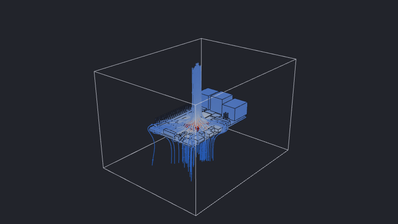
Temperature-colored bare Raspberry Pi 5 with streamlines rising from the exposed BCM2712 through the open-air domain. — Bare-board solid temperatures and natural-convection streamlines on the complete 20.0–287.8 °C computed range. The box is the open-air fluid domain; show the fluid mesh to inspect its exterior cells.

Raspberry Pi defines a hard thermal limit of 85 °C, with throttling beginning at 80 °C. The solve finishes with max_iterations_reached and the BCM2712 already at 284.83 °C. Its final 20 junction samples span 0.176 °C, but the configuration is already clearly unfit, so we do not continue toward full convergence.

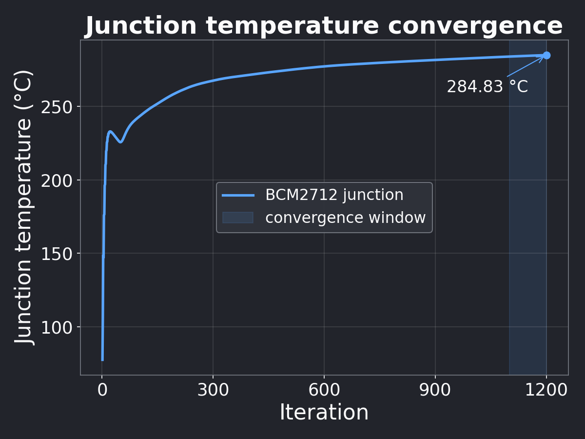
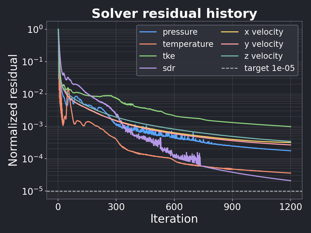
BCM2712 junction-temperature history rising to 284.83 degrees Celsius over the capped 1200-iteration natural-convection solve. — At the fixed 8.6 W board load, natural convection alone does not provide an adequate heat path.

Logarithmic pressure, temperature, turbulent kinetic energy, specific dissipation rate, and velocity residual histories for the capped 1200-iteration natural-convection solve. — Residual history over the capped 1,200 iterations.

That extreme temperature is not a realistic operating prediction: a physical Pi would throttle or shut down first, and the model assumptions become less reliable across such a large temperature rise. This clearly shows that the Pi needs active cooling at this operating point.

3. Add the Active Cooler

This need is reflected in the real hardware. For sustained heavy loads, Raspberry Pi produces a purpose-built Active Cooler for the Raspberry Pi 5. Its aluminum base and 54 fins form one connected solid, paired with a side-exhaust blower.

We add this cooling assembly while keeping every baseline input fixed, so the second run isolates its effect. Conducting pads fill the gaps from the SoC, RP1, PMIC, and wireless shield to the flat cooler underside. Heat enters through these pads, spreads through the base, and reaches the airflow through the fins; without the pads, small air gaps would break this conduction path.

The fan is represented by an annular intake on the top face of a 30 mm box and a rectangular exhaust on its x_min side face, directed through the fin bank. Its 25 mm opening, 15 mm hub, and nine-point fan curve are the ones tested in the earlier fan-only case. Here the intake and exhaust are linked across an internal blower component rather than placed on the external domain.

4. Run the cooled Pi

Download raspberry-pi-5-active-cooler.json and submit it with the same API workflow:

curl -i -X POST \
  https://api.vanellus.tech/simulations \
  -H "Content-Type: application/json" \
  -H "X-API-Key: $VANELLUS_API_KEY" \
  --data-binary @raspberry-pi-5-active-cooler.json

Or reuse the Python package and change only the cooler flag:

python raspberry_pi_5_cooling.py --active-cooler --name active-cooler

To inspect the cooled mesh before starting the full simulation, run:

python raspberry_pi_5_cooling.py --active-cooler --dry-run --name active-cooler-mesh

This detailed solve also uses credits. Unlike the failed baseline, it runs until the junction temperature is stable.

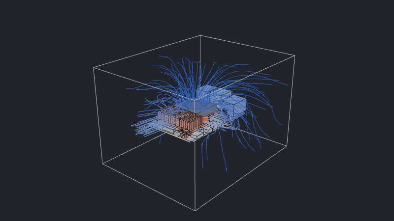
Temperature-colored Raspberry Pi 5 and Active Cooler with streamlines leaving the blower and passing through the fin bank. — Active Cooler solid temperatures on the complete 20.0–77.1 °C solved range; the box is the fluid domain.

The gray box is the blower. The darker annulus marks its intake, and the matching rectangle marks the side exhaust that blows through the heatsink pins.

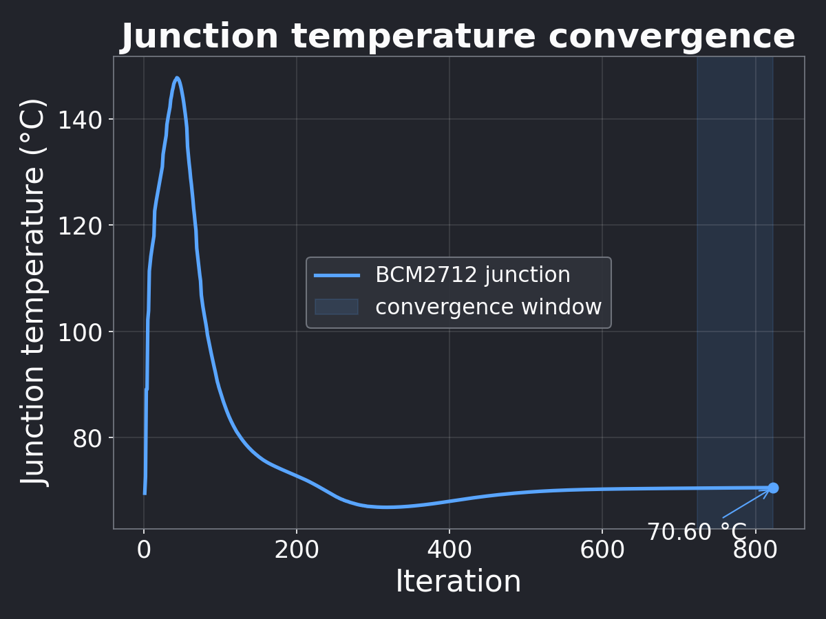
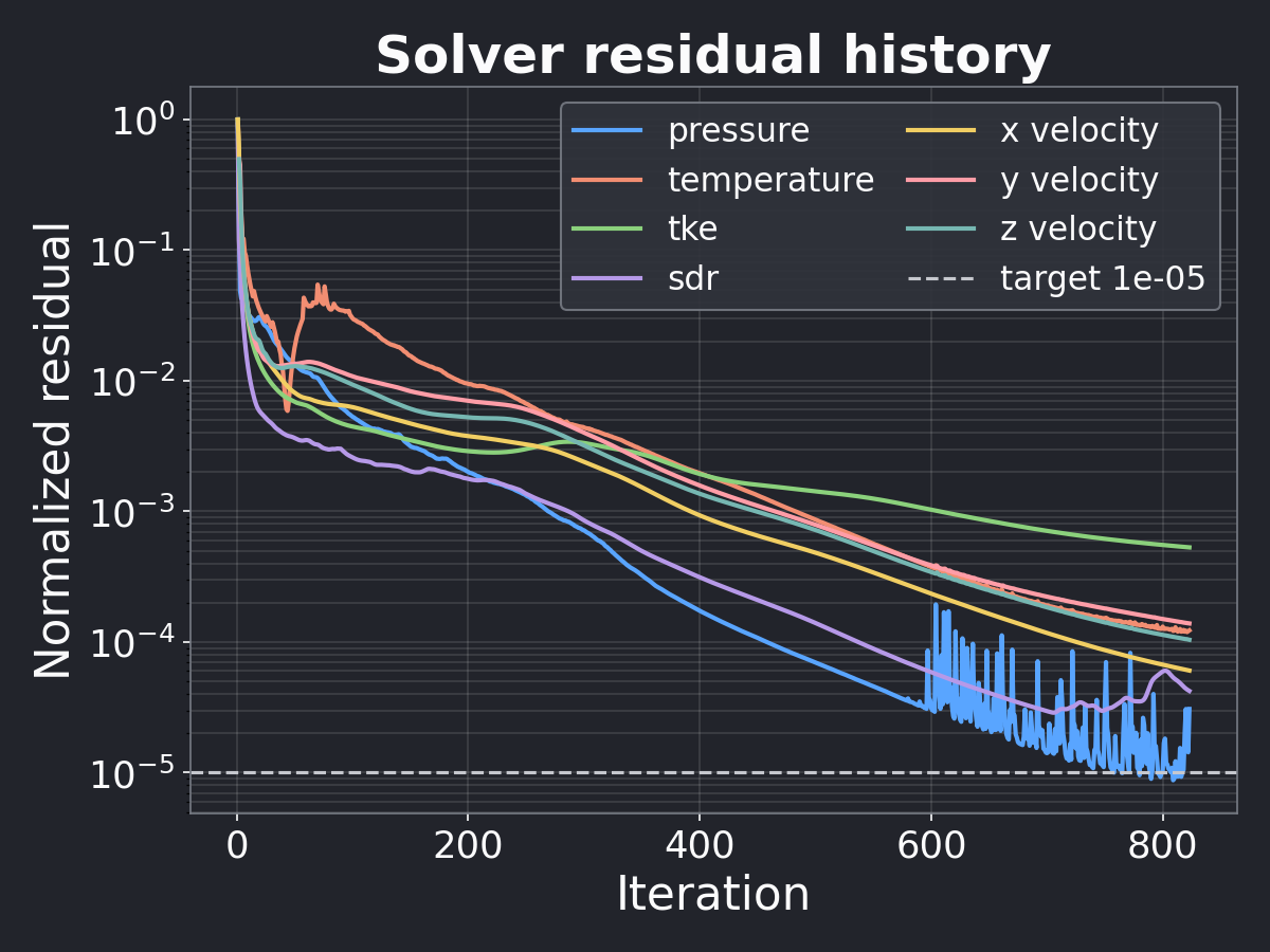
Over the final 100 iterations, the greatest deviation from the window mean is 0.0497 °C, just below the 0.05 °C tolerance. The residuals are still decreasing, but junction temperature stability is the stopping condition for the cooled run:

BCM2712 junction-temperature history settling at 70.60 degrees Celsius, with the final 100-iteration convergence window shaded. — The BCM2712 junction-temperature criterion stops the solve at 70.60 °C.

Logarithmic pressure, temperature, turbulent kinetic energy, specific dissipation rate, and velocity residual histories over 823 iterations. — Residual history from the validated whole-board solve.

5. Compare the results

Configuration	Cells	Iterations	BCM2712 junction
Natural convection	1,545,859	1,200 cap	284.83 °C
Active Cooler	3,016,080	823	70.60 °C

Adding the Active Cooler reduces the predicted BCM2712 junction temperature by 214.23 °C in this controlled model. The cooled result settles at 70.60 °C—14.40 °C below the 85 °C limit and 9.40 °C below the 80 °C point where throttling begins. Because the board load, ambient conditions, and component models are unchanged, the comparison isolates the improvement made by the cooler: it provides the missing path from the SoC into the air and keeps the junction within its operating range at this load.

The result is therefore more than a lower temperature. Within the assumptions of this model, the bare Pi cannot sustain the chosen maximum operating point, while the Active Cooler can. That is the design decision this pair of simulations was built to answer.

Take the workflow further

Across this tutorial, we progressed from flow through an empty duct to conjugate heat transfer, compact thermal models, fans, CAD heatsinks, and finally a complete board-level comparison. We can now turn a cooling question into a model, establish a baseline, change one part of the thermal solution, and judge the result from both convergence and the required temperature limit.

The Python case package also provides a ready-made test bed for further experiments, such as:

varying the fin height, spacing, orientation, or base thickness in the cooler STEP file;
designing a different active cooler for the same board and thermal pads;
adjusting the cooler fan curve to explore different airflow performance.

Each variation can be assessed against the 70.60 °C baseline while keeping the Pi and operating point fixed.

For a new case, the How-to guides cover focused modeling and result tasks, while Explanation describes the underlying Vanellus models and solver behavior.

Keyboard shortcuts

Vanellus Guide