Model a chip with a compact thermal model
On this page, we will replace the generic powered block with a PCB and a two-resistor chip package, then run until the predicted junction temperature settles. The package is inspired by the Raspberry Pi 5’s BCM2712 SoC and uses the same 6 W compact thermal model that we will later place on the complete board. This creates the baseline for our 80 °C design goal; the next two stages will improve the same heat path.
This page is part of Design a complete electronics cooling solution.
Choose how to start:
- Start with multiple-components.json from the
previous tutorial. Copy it and rename the copy
compact-thermal-model.json. - Skip the edits on this page and download the completed compact-thermal-model.json, then continue with Check the contacts.
1. Resize the duct and add the PCB
Open compact-thermal-model.json and change domain.size to a 120 × 70 × 25 mm duct:
"size": [0.12, 0.07, 0.025]
Remove the existing inlet_step and block entries from cuboid_components, then restore the full-face inlet:
{
  "boundary": { "full": { "side": "x_min" } },
  "condition": {
    "velocity_inlet": {
      "speed": 0.5,
      "temperature": 20.0
    }
  }
}
Replace cuboid_components with this PCB:
"cuboid_components": [
  {
    "tag": "pcb",
    "bbox": {
      "origin": [0.0175, 0.007, 0.0],
      "size": [0.085, 0.056, 0.0016]
    },
    "thermal_model": {
      "conducting": {
        "conductivity": [10.0, 10.0, 0.3],
        "density": 1850.0,
        "specific_heat_capacity": 1100.0,
        "power": 0.0
      }
    }
  }
]
The PCB now rests on the lower duct wall.
2. Add the chip package
Append this component to cuboid_components:
{
  "tag": "chip",
  "bbox": {
    "origin": [0.0555, 0.027, 0.0016],
    "size": [0.016, 0.016, 0.0022]
  },
  "thermal_model": {
    "two_resistor_ctm": {
      "case_side": "z_max",
      "power": 6.0,
      "resistance_jb": 9.2,
      "resistance_jc": 0.5,
      "exit_tolerance": 0.05
    }
  }
}
The simplified package sits directly on the PCB, with its z_max case face exposed to the air. Its dimensions suit this small tutorial duct; its power and junction-to-board and junction-to-case resistances match the BCM2712 model used in the final Raspberry Pi case. Its two heat paths are shown below:
For more detail on this representation, see Conducting and insulating domains. Model an electronic package with a compact thermal model gives the focused procedure for two-resistor and star-resistor packages.
3. Check the contacts
Update the top-level run settings:
"max_iterations": 500,
"target_residual": 1e-7,
"convergence_window": 20,
"numerics": "balanced",
"mesh_settings": {"max_cell_size": 0.002},
"boussinesq": true,
"gravity": [0.0, 0.0, -9.81],
"ctm_coupling": "implicit"
Compare the request with the completed compact-thermal-model.json, then submit a dry run and download its result.
This case includes Boussinesq buoyancy. Boussinesq buoyancy and reference temperature explains the model and its API inputs.
Inspect the geometry in fluid.vtu and solid.vtu with any compatible viewer. Check that:
- the PCB forms one continuous layer inside the duct;
- the package sits directly on the PCB without a gap or overlap;
- the complete lower package face contacts the PCB; and
- the complete upper package face contacts the fluid.
Correct the component bounding boxes before continuing if any contact is wrong.
Boundary placement and defaults explains why these contacts determine the available heat paths.
4. Run until the chip temperature settles
Set dry_run to false, submit the request, and download the result. The validated 30,744-cell case stops with monitor_converged after 80 iterations.
Open iteration_info.csv and inspect the final rows of junction_temperature_chip:
This preview shows a subset of the rows and columns in iteration_info.csv.
iteration | junction_temperature_chip |
|---|---|
| … | … |
| 78 | 254.85693 |
| 79 | 254.85806 |
| 80 | 254.85846 |
The chip temperature has flattened within the configured 20-iteration window.
Monitor a result and stop when it settles covers choosing a convergence window and tolerance for an engineering quantity.
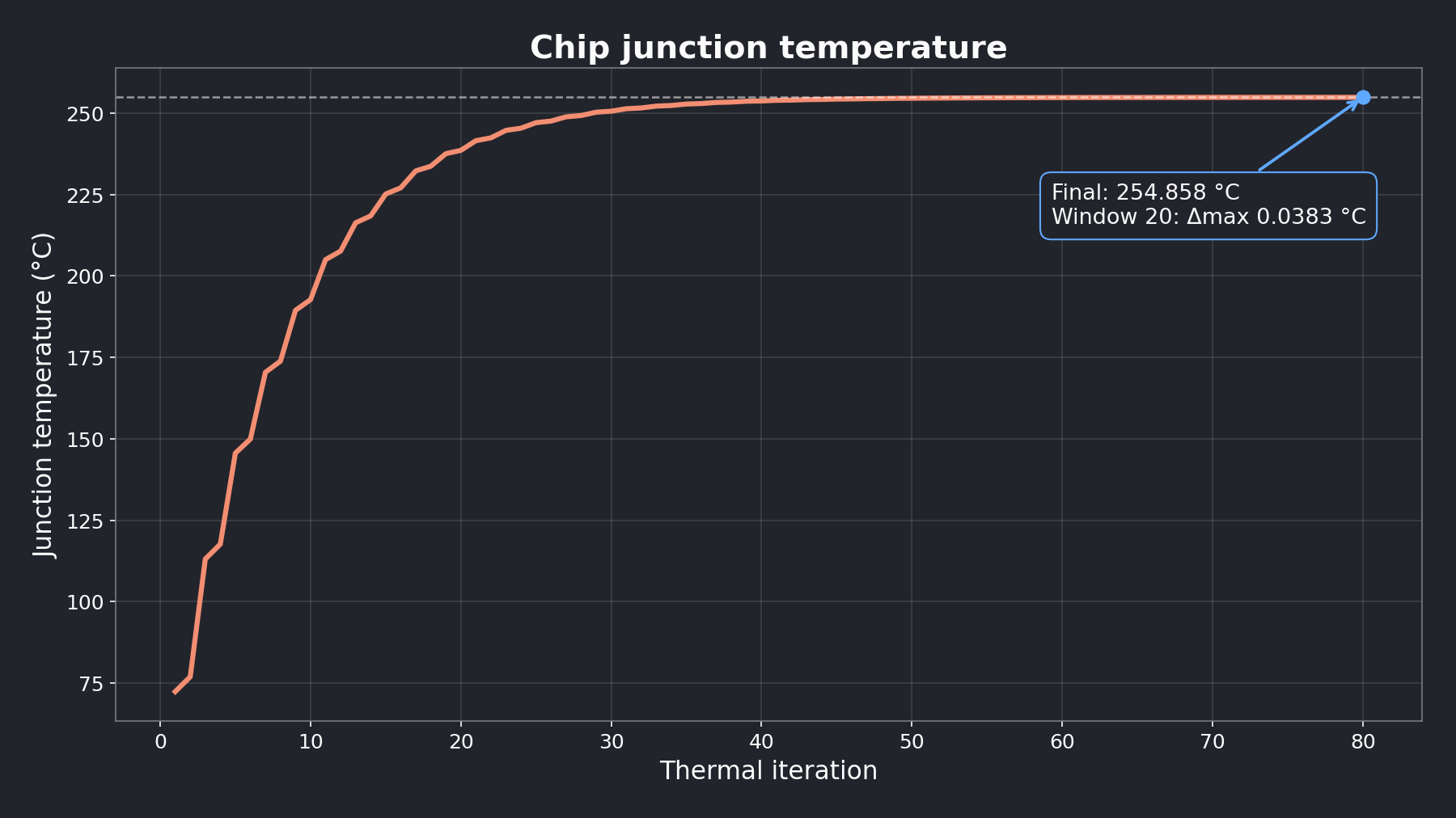
254.858 °C is far above the 80 °C goal and indicates an unsuccessful thermal strategy. That is still a useful result: it gives us a converged baseline and identifies the missing path from the package into the air. Convergence means the result has stopped changing; it does not mean the design is thermally acceptable. Compare a real result with the chip manufacturer’s maximum junction temperature.
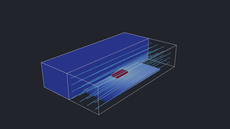
Inspect the solved speed and temperature fields with a VTU viewer. We should see the chip as the hottest region, with a cooler PCB and airflow around it. In the interactive result, the PCB and chip are complete but only the back half of the fluid field is displayed. The front half is cut away at the duct center plane; the white box marks the complete fluid domain used by the simulation. Blue arrowed streamlines begin at the uniform inlet and follow the solved airflow. Open Display and uncheck Fluid to expose the complete solids, or Streamlines to hide the airflow paths. The optional ParaView workflow explains how to build a similar view.
Finally, use the residual_* columns in iteration_info.csv to confirm that the pressure, velocity, and temperature residuals decrease across the run.
This preview shows a subset of the rows and columns in iteration_info.csv.
iteration | residual_pressure | residual_temperature |
|---|---|---|
| 1 | 1 | 1 |
| 2 | 0.13051555 | 0.16442731 |
| … | … | … |
| 79 | 0.0003380445 | 0.000016483013 |
| 80 | 0.00026254207 | 0.000008906038 |
Baseline established
We:
- added a conducting PCB;
- attached a two-resistor chip model to it;
- checked the package contacts with a dry run; and
- stopped a full simulation using the junction-temperature history.
The key result is the 254.858 °C baseline. The model has a source, a junction monitor, and valid thermal contacts; what it lacks is adequate cooling. Next, we will cool the chip with an annular fan and test whether faster air alone can close the gap to 80 °C.