Explore flow through a heated duct
This is the baseline for Design a complete electronics cooling solution. We will create a small heated duct request from scratch and complete the edit–submit–inspect loop that every later design change reuses. Its solved flow and thermal fields give the later electronics cases a controlled foundation.
We will:
- create a JSON file representing a heated duct simulation
- inspect the meshed geometry using
dry_run - submit the request to the Vanellus solver API
- inspect the resulting speed, pressure, and temperature fields
The commands require an API key available as VANELLUS_API_KEY. Use Set up API access and Use the key from a terminal if it is not configured yet.
We will also need a text editor and a terminal with curl. Check that curl is available by running curl --version; the command should print a version number. The interactive reference results on this page show the fields we should expect. To explore the downloaded VTU files, use any compatible viewer or follow the optional ParaView workflow.
1. Define the duct
We will define an air-filled rectangular duct with an inlet on the x-min face and an outlet on the x-max face. The bottom, z-min wall has a fixed temperature; the remaining walls are adiabatic, which means that no heat passes through them. There are no internal solid components.
The schematic shows how the geometry, boundary conditions, and coordinate axes relate to one another:
For this simulation, we will use the following parameters:
| Parameter | Value |
|---|---|
| Origin (x, y, z) | [0, 0, 0] m |
| Size (x, y, z) | [0.10, 0.02, 0.02] m |
| Air at the x-min inlet | 0.5 m/s at 20 °C |
| Static pressure at the x-max outlet | 0 Pa |
| Temperature of the z-min wall | 30 °C |
Create a new directory for the tutorial, open it in a terminal, and save the following as heated-duct.json. The JSON file is also available to download.
{
  "dry_run": true,
  "domain": {
    "origin": [0.0, 0.0, 0.0],
    "size": [0.1, 0.02, 0.02],
    "boundary_conditions": [
      {
        "boundary": {
          "full": {
            "side": "x_min"
          }
        },
        "condition": {
          "velocity_inlet": {
            "speed": 0.5,
            "temperature": 20.0
          }
        }
      },
      {
        "boundary": {
          "full": {
            "side": "x_max"
          }
        },
        "condition": {
          "static_pressure_outlet": {
            "pressure": 0.0
          }
        }
      },
      {
        "boundary": {
          "full": {
            "side": "z_min"
          }
        },
        "condition": {
          "fixed_temp": {
            "temperature": 30.0
          }
        }
      }
    ]
  },
  "fluid_properties": {
    "air": {}
  },
  "max_iterations": 100,
  "target_residual": 0.01,
  "numerics": "fast",
  "mesh_settings": {
    "max_cell_size": 0.002
  },
  "turbulence_model": "navier_stokes",
  "boussinesq": false,
  "ctm_coupling": "implicit"
}
The domain object defines the duct’s origin, size, and boundary conditions. In Vanellus, every boundary is an adiabatic wall by default. The boundary_conditions array overrides that default on three faces: it sets the x-min face as the velocity inlet, the x-max face as the static-pressure outlet, and the bottom z-min face as the fixed-temperature wall. The other three faces keep the default adiabatic-wall condition.
Geometry and the computational domain and Boundary placement and defaults describe what these choices represent. When adapting the case, use Set the computational domain, then refer to Flow boundary conditions and Thermal boundary conditions for the available inputs.
The remaining mesh, solver, and numerical settings keep this baseline small and quick to solve; leave them unchanged for now.
2. Send a dry-run request
Dry runs are not sent to a GPU worker, so they do not spend solver credits. Use them while setting up a case: inspect the geometry and mesh with dry runs, then submit a full simulation when the case is ready. Configure the mesh shows the mesh settings for resolving smaller features.
We will use the API’s Start simulation request. It is an HTTP POST to /simulations:
- the URL identifies the action;
- the
X-API-Keyheader identifies our account; and heated-duct.jsonis the request body describing the simulation.
From the directory containing heated-duct.json, run:
curl -i -X POST \
  https://api.vanellus.tech/simulations \
  -H "Content-Type: application/json" \
  -H "X-API-Key: $VANELLUS_API_KEY" \
  --data-binary @heated-duct.json
The @ in @heated-duct.json tells curl to use the contents of that file as the request body. Keeping the request in a separate file makes it easy to edit and submit again.
The -i option includes the HTTP status and headers in the output. After those headers, the returned JSON should contain an id field, such as "id": 123. The ID will be different. Note it for the next step.
3. Download the dry-run files
Open Simulations in the dashboard. The page does not update automatically, so refresh it to see the latest simulations and their current states. Find the row whose simulation ID matches the id returned by curl. A small dry run may complete before the page first loads. Once it is complete, its status reads Dry run and the row has a Download action.
Download and extract the ZIP archive. For the dry run, we only need to look at the VTU files: fluid.vtu and solid.vtu.
Simulation status and result files explains how job states and downloaded artifacts relate.
4. Inspect the mesh
Inspect fluid.vtu with a VTU-compatible viewer. The result is a 100 mm × 20 mm × 20 mm rectangular duct made from 5,000 fluid cells.
solid.vtu contains 0 cells because our request did not define any internal solids. Vanellus includes both domain files so the result bundle has the same structure for fluid-only and conjugate heat-transfer simulations.
With a compatible viewer, inspect speed. The duct should be a single color because the dry-run velocity is zero throughout the domain. Velocity, pressure, and temperature are all placeholder fields at this stage: we built the mesh, but did not solve the equations.
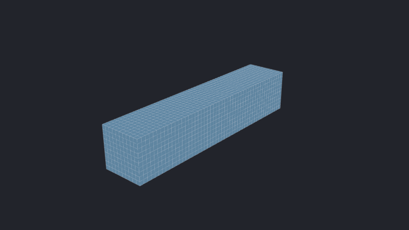
Checkpoint: we have validated the domain and mesh without spending solver credit. Keep this habit: geometry first, physics second.
5. Experiment with the geometry
In heated-duct.json, find the domain size:
"size": [0.1, 0.02, 0.02]
The three values are the duct dimensions in the x, y, and z directions, measured in meters. Change one or more of them to adjust the size of the domain. Keep max_cell_size unchanged so that this experiment remains small.
Save the file, repeat the same curl command, then download and inspect the new fluid.vtu. Notice how the duct has changed in size. Check how many cells the new mesh contains and compare it with the 5,000 cells in the original 100 mm × 20 mm × 20 mm duct.
We can repeat this experiment with another size. Each dry run follows the same API workflow: edit the JSON, submit it, and inspect the result.
Before running the solver, restore the original size so that the full simulation uses the small case we have already validated:
"size": [0.1, 0.02, 0.02]
6. Run the simulation
Unlike a dry run, a full simulation is sent to a GPU worker and uses solver credits. This case is deliberately small, so the solver should need only a few seconds of GPU time.
Change the dry_run setting at the top of heated-duct.json from:
"dry_run": true
to:
"dry_run": false
Save the file and run the same request again:
curl -i -X POST \
  https://api.vanellus.tech/simulations \
  -H "Content-Type: application/json" \
  -H "X-API-Key: $VANELLUS_API_KEY" \
  --data-binary @heated-duct.json
The response contains a new simulation ID for the full run.
Open the Simulations dashboard again and find that ID. The page does not live update, so refresh it to see the current state. While the solver is working, its status shows Running; it may have finished before we open the page, because this simulation is intentionally small in order to run very quickly. The validated case finishes with residual_converged after about 49 SIMPLE iterations, although the exact count can vary.
7. Inspect the solved result
Download and extract the completed simulation, keeping it separate from the dry-run files.
Open iteration_info.csv. It contains one row per SIMPLE iteration; the residual_* columns include pressure and the three velocity components:
This preview shows a subset of the rows and columns in iteration_info.csv.
iteration | residual_pressure | residual_x_velocity | residual_y_velocity | residual_z_velocity |
|---|---|---|---|---|
| 1 | 1 | 1 | 0 | 0 |
| 2 | 0.16518407 | 0.6303875 | 0.4847205 | 0.48472047 |
| … | … | … | … | … |
| 48 | 0.0045465524 | 0.0013522652 | 0.010702223 | 0.010702212 |
| 49 | 0.0038389154 | 0.0010985034 | 0.009075354 | 0.00907537 |
The values record how the flow-equation residuals changed as the solver approached the target_residual of 0.01 set in heated-duct.json. At iteration 49, every residual was below 0.01, so the solver stopped; the generated table shows the preceding values for comparison. Residuals and linear-solver convergence explains how these values are scaled and how they differ from the residual used inside each linear solve.
This stopping condition shows that the numerical iteration settled; it does not validate the model or its result.
Inspect the solved fields in fluid.vtu with a compatible viewer. Look for:
- speed, calculated from
velocity, which varies through the duct and slows near the walls; pressure, which falls from the inlet toward the 0 Pa outlet; andtemperature, which rises from the 20 °C inlet air toward the 30 °C lower wall.
In the speed field, air away from the walls should move faster than air beside them. In the temperature field, the hottest air should lie beside the fixed-temperature z_min wall. Use the field selector in the interactive reference result to compare those patterns directly.
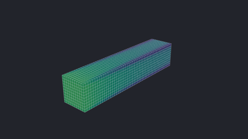
Unlike the dry-run fields, these fields are not uniform. They are the result of the completed solve. solid.vtu still contains 0 cells because changing from a dry run to a solve does not change the geometry.
Duct baseline complete
We completed the edit–submit–inspect loop reused by the later stages:
- Described a CFD simulation in JSON.
- Submitted the request as both a dry run and a full solve.
- Followed both simulations on the dashboard.
- Downloaded and interpreted the mesh and solved fields.
The mesh is unchanged, but solving creates a wall-bounded speed profile and carries heat from the lower wall into the air. Next, add solid components to the duct and turn this fluid-only case into a conjugate heat-transfer model.