Add solid components to the duct
On this page, we will add an insulating block to a heated duct, make it conducting and powered, then add an insulating inlet step. Each change answers a different modeling question: where can air flow, where can heat flow, and how do components reshape both paths?
This page is part of Design a complete electronics cooling solution.
Choose how to start:
- Start with heated-duct.json from the previous tutorial. Copy it
and rename the copy
solid-components.json. - Skip the edits on this page and download the completed multiple-components.json.
For the focused procedure and placement rules, see Add a cuboid component.
1. Add an insulating block
Open solid-components.json and add this cuboid_components array at the top level, alongside
domain and fluid_properties. The starting request already has dry_run set to true:
"cuboid_components": [
  {
    "tag": "block",
    "bbox": {
      "origin": [0.04, 0.005, 0.006],
      "size": [0.02, 0.01, 0.008]
    },
    "thermal_model": "insulating"
  }
]
Compare the edit with the completed insulating-component.json, then
submit solid-components.json:
curl -i -X POST \
  https://api.vanellus.tech/simulations \
  -H "Content-Type: application/json" \
  -H "X-API-Key: $VANELLUS_API_KEY" \
  --data-binary @solid-components.json
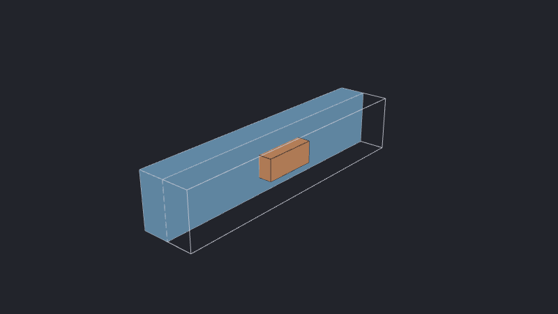
Download and inspect fluid.vtu and solid.vtu. The block should occupy a cavity in the fluid
without touching the duct walls.
How to read these views: the solid geometry is always shown in full, but only the back half of the fluid field is displayed. The front half is cut away along the duct center plane so the solid and the flow immediately around it remain visible. This is only a visualization cutaway: the simulation still uses the complete fluid domain marked by the white box. Open Display and uncheck Fluid to inspect the unobscured solid.
The first interactive reference applies this cutaway to the dry-run fluid mesh. To reproduce that view locally, follow the optional ParaView workflow.
Set dry_run to false and submit the request again. The validated case finishes with residual_converged after 22 iterations.
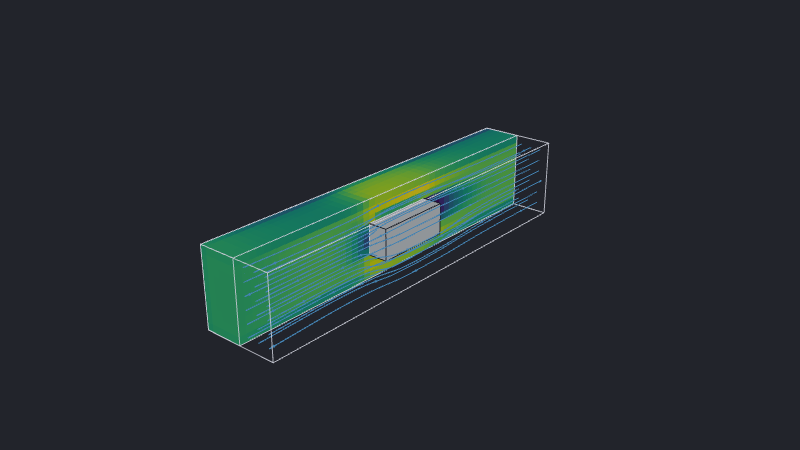
Inspect speed and temperature with a viewer that supports field data. We should see faster flow around the block and a wake behind it. The fluid warms around the obstruction, but the insulating block has no solved temperature and should remain neutral. The field selector in the reference result shows both patterns. Blue arrowed streamlines trace the flow through the complete duct; uncheck Streamlines under Display to hide them.
Conducting and insulating domains explains why insulating and conducting solids produce different temperature fields.
2. Make the block conducting and powered
In the same working file, replace "thermal_model": "insulating" with:
"thermal_model": {
  "conducting": {
    "conductivity": 0.5,
    "density": 2700.0,
    "specific_heat_capacity": 900.0,
    "power": 1.0
  }
}
Compare the request with conducting-component.json. Set dry_run to false, submit it, and download the result. The validated case finishes with residual_converged after 32 iterations.
Inspect the fluid and solid temperatures using one shared range in a viewer that supports it. The block should be hottest in its interior and cooler at its surfaces. The interactive result below provides the same comparison without requiring any viewer setup.
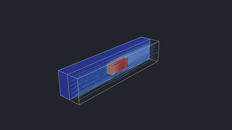
Compare this result with the insulating case. Changing thermal_model determines whether the component participates in the thermal solve. The geometry still obstructs the flow, but the conducting block now has a solved internal temperature gradient and transfers its 1 W load into the surrounding air. Also note that the lower fixed temperature boundary still heats up the flow,
but the conducting block now dominates.
Conducting and insulating domains explains when component temperatures are solved.
3. Add an inlet step
Continue with the conducting-block request and make these changes:
- Remove the fixed-temperature lower-wall condition.
- Replace the full-face inlet with the rectangle below.
- Replace
cuboid_componentswith the following two-component array.
The rectangular inlet leaves the lower 8 mm for the insulating step:
Select a boundary region covers the coordinate order and mesh controls for full, rectangular, and other shapes of boundary regions.
{
  "boundary": {
    "rectangle": {
      "center": [0.01, 0.014],
      "size": [0.02, 0.012],
      "side": "x_min"
    }
  },
  "condition": {
    "velocity_inlet": {
      "speed": 0.5,
      "temperature": 20.0
    }
  }
}
Use this component array:
"cuboid_components": [
  {
    "tag": "inlet_step",
    "bbox": {
      "origin": [0.0, 0.0, 0.0],
      "size": [0.02, 0.02, 0.008]
    },
    "thermal_model": "insulating"
  },
  {
    "tag": "block",
    "bbox": {
      "origin": [0.04, 0.005, 0.006],
      "size": [0.02, 0.01, 0.008]
    },
    "thermal_model": {
      "conducting": {
        "conductivity": 0.5,
        "density": 2700.0,
        "specific_heat_capacity": 900.0,
        "power": 1.0
      }
    }
  }
]
Compare the request with multiple-components.json, then submit a dry run. Confirm that:
- the inlet contains fluid only above the step;
- the two solids do not overlap; and
- an open fluid path remains to the outlet.
Use the controls in Configure the mesh if a component, clearance, or boundary patch is represented poorly.
Set dry_run to false and submit the request again. The validated case finishes with residual_converged after 31 iterations.
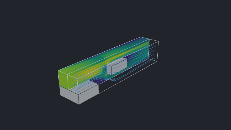
Inspect speed and temperature in the downloaded fields with a compatible viewer. As above, the interactive result keeps only the back half of the fluid field around the complete solids. The streamlines make it possible to match the accelerated path with the thermal wake.
The residual history for this run is shown below.
This preview shows a subset of the rows and columns in iteration_info.csv.
iteration | residual_pressure | residual_x_velocity | residual_y_velocity | residual_z_velocity |
|---|---|---|---|---|
| 1 | 1 | 1 | 0 | 0 |
| 2 | 0.22372937 | 0.5026472 | 0.38485456 | 0.40365815 |
| … | … | … | … | … |
| 30 | 0.0110406075 | 0.0038249888 | 0.0068233768 | 0.0058525684 |
| 31 | 0.009927777 | 0.0033008466 | 0.0053809737 | 0.004752265 |
What we learned
We:
- added and positioned insulating and conducting cuboids;
- checked component placement with dry runs;
- inspected speed and temperature results; and
- restricted an inlet around a solid component.
We can now separate three roles in an electronics model: insulating geometry shapes the flow, conducting geometry carries heat, and boundary regions determine where the fluid enters. Next, we will model a chip with a compact thermal model and replace the generic powered block with an engineering junction-temperature prediction.