Rectilinear meshing
Vanellus uses a rectilinear finite-volume mesh. Every cell is an axis-aligned cuboid, and so its width can vary independently along each axis. This representation is an important difference from an unstructured mesh, an octree mesh, or a Cartesian mesh with independently refined zones.
Cells, nodes and mesh planes
A node is a point at a cell corner. A cell is a cuboid volume with eight corner nodes and six faces. Neighbouring cells share the nodes on their common face.
The mesher produces one ordered array of node coordinates for each axis:
\[ x_0, x_1, \ldots, x_{N_x} \qquad y_0, y_1, \ldots, y_{N_y} \qquad z_0, z_1, \ldots, z_{N_z} \]
Choosing two adjacent coordinates on each axis defines a cell: their eight combinations give its corner nodes. Each axis has one more node coordinate than it has cell intervals. The complete mesh therefore contains
\[ N_{\mathrm{cells}} = N_x N_y N_z \]
cells before solid and fluid labels divide them into separate result files.
A mesh plane is formed by fixing one axis at a node coordinate and spanning the other two axes. For example, fixing x gives a y–z plane through the whole domain. Fixing y or z similarly gives an x–z or x–y plane. These planes form the mesh lines seen in a two-dimensional cross-section.
Unlike a block-structured or adaptive rectilinear mesh, Vanellus does not introduce independent subgrids whose node lines can end at a refinement-zone boundary. All cells use the same three coordinate arrays.
Example: refine a central component
To see how this affects a mesh, consider a 20 mm cuboid inside a 120 × 80 × 40 mm domain. The first mesh uses a 10 mm global cell-size limit and no local limit on the component. Its faces are still fitted by the mesh. The three arrays contain 14, 9, and 5 nodes, producing 13 × 8 × 4 = 416 cells.
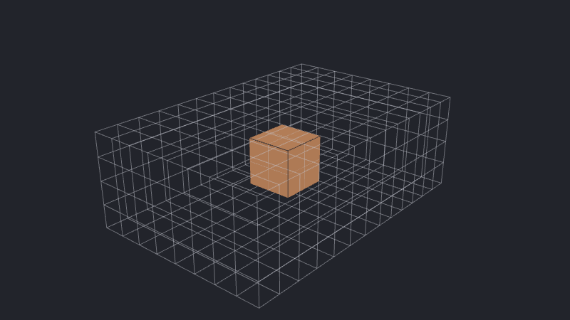
A component max_cell_size applies inside that component’s bounding region. It tells the mesher where finer spacing is required, but it does not create an isolated block of finer cells.
When the central cuboid requests a 1 mm maximum cell size, the mesher adds extra coordinates along its x, y, and z extents. Each new coordinate continues through the domain as a complete plane. Their intersections create bands of smaller cells outside the cuboid as well as inside it.
In addition, the mesher enforces a smooth growth in the cell sizes (controlled by max_growth_rate and boundary_layer_growth_rate), meaning the refined region near the solid extends outwards as the cells grow to their maximum size.
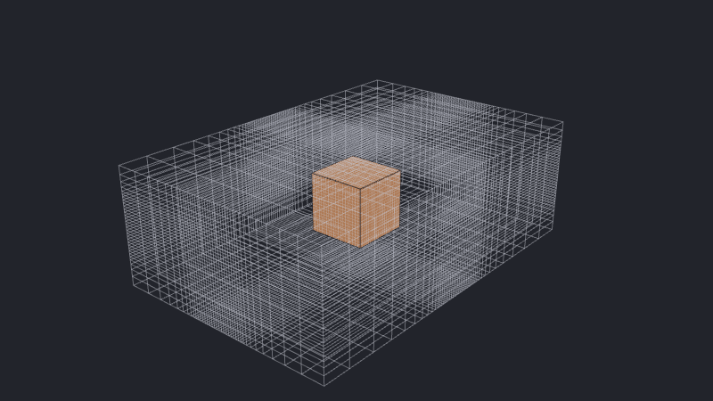
The refined mesh has 42, 38, and 32 nodes, producing 41 × 37 × 31 = 47,027 cells. Only 8,000 are solid component cells; the other 39,027 are fluid cells created by the same axis arrays. In this sense, local describes where a spacing requirement originates, not where every resulting fine cell remains.
Ramifications for mesh design
This structure changes how refinement costs should be anticipated:
- Adding nodes on one axis increases the number of cells across both other axes. Refining x, y, and z together multiplies those increases.
- Several small features at different x, y, and z positions can combine their node planes and create many cells between the features. Removing unnecessary features (such as small screws or solder) or adjusting alignments can help with this issue. This can be done automatically for
cuboid_componentsby increasingbbox_cull_threshold. - Tiny gaps, thin parts, detailed CAD vertices, and small boundary patches can affect more of the mesh than their physical volume suggests. Small gaps can be removed by increasing the
fuse_threshold. - Directional
[x, y, z]cell-size limits can avoid resolving an axis more finely than the geometry or physics requires.
This does not mean local refinement should be avoided. It means the cell count and resulting mesh should be inspected after adding each important sizing constraint.
Why Vanellus uses a rectilinear mesh
The regular indexing gives the GPU predictable neighbours and memory access without storing and traversing the connectivity used by an unstructured mesh. That suits the solver’s numerical kernels, linear algebra, and multigrid operations, allowing high per-cell throughput. In addition, rectilinear mesh generation is order-of-magnitudes faster than unstructured mesh generation due to the fact it is defined by just three 1D arrays.
The trade-off is that a rectilinear mesh can need more cells to resolve a local feature than an unstructured or independently refined mesh. Those extra cells do not necessarily make the solve slower overall; in fact, at a given resolution a rectilinear mesh can result in faster runtimes despite the increased cell-count because the underlying data structures are better suited to GPU operations.
See also
- CAD voxelization shows how this mesh represents imported surfaces, including curved and rotated parts.
- Mesh resolution and controls explains how the mesher combines its constraints.
- Configure the mesh shows how to apply the mesh controls.