Run your first simulation with Python
Run an electronics-cooling simulation with the Vanellus API and inspect its predicted chip temperature.
The model represents a 90 W NVIDIA Jetson Thor chip on a PCB beneath a heat spreader and thirteen-fin heatsink. A circular fan inlet supplies 20 °C air.
Prepare Python
Complete Set up API access, then check that the key is available without printing it:
test -n "$VANELLUS_API_KEY" && echo "API key is ready"
Create a new directory and download jetson_cooling.py into it. From that directory, install the client dependencies:
python -m pip install requests matplotlib
Run the simulation
This is a full solver run and uses credits. Start it with:
python jetson_cooling.py
The client submits the case, prints progress while it runs, and downloads the completed result into results/simulation-<id>.
When the solve finishes, it reports the predicted junction temperature:
Simulation finished with status monitor_converged
Jetson junction temperature: 73.7 °C
The Jetson is below the 80 °C tutorial target.
For this case, the validated run stops after 174 iterations when its junction temperature has settled.
Inspect the result
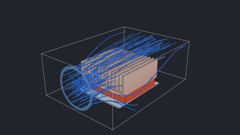
The result directory contains the submitted request, convergence history, plots, and VTU fields. Start with junction-temperatures.png and residuals.png to check how the result settled. Use Inspect simulation results in ParaView to explore the spatial fields.
Change the simulation
The first run gives us a baseline. Next, change the heatsink and chip power and compare the new junction temperature against that baseline.
The inputs used by the model are constants near the top of the file:
# Keep commonly changed physical inputs together as ordinary Python values.
JETSON_POWER_W = 90.0
NUM_FINS = 13
The client exposes these as command-line options. Run a named variant with fewer fins and a higher chip power:
python jetson_cooling.py --num-fins 9 --jetson-power 100 --name nine-fins
This submits another full simulation, uses credits, and writes the result to results/nine-fins. Compare its junction-temperature and residual plots with the baseline.
We can make the same change in Python when building a request:
request = build_request(
    jetson_power=100.0,
    num_fins=9,
)
Alternatively, edit JETSON_POWER_W or NUM_FINS and rerun the file. The heatsink function calculates evenly spaced fin positions and adds the resulting components to the request.
Constructing the request in Python lets values, calculations, functions, and loops change the model without duplicating fields in raw JSON. To vary another property, add it as an argument to the function that builds that part and pass it through build_request. The same approach works for dimensions, materials, boundary conditions, and solver settings.
What we accomplished
We used Python to:
- construct an electronics-cooling request from reusable functions;
- submit it with an API key;
- follow its progress and lifecycle status;
- download its result files;
- plot its residual and junction-temperature histories; and
- change model inputs without editing raw JSON.
Continue with Design a complete electronics cooling solution to construct a model from an empty duct. Use Automate a simulation with Python when adapting the reusable API and result-handling workflow for a new model.